Notes about feed forward and back proporgation for neural network
Feed forward and back proporgation is widely used to train a neural network model. Specifically, feed-forward step passes the input into the model to calculate the value of neurons in each layer. After feed-forward, neuron values reversely give us the ‘error’ of each neuron and further the gradient of each parameters from far to near layers, which is called back proporgation.
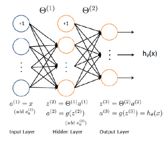
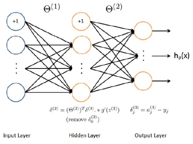
Below is a neural network model (img from Week5, Machine Learning in Coursera).


Weights for layer \((l)\) \(\mathbb{\Theta}^{(l)} \in \mathbb{R}^{s_l\times s_{l+1}}\). Design matrix \(X \in \mathbb{R}^{m\times n+1}\) where m is the number of sample and n is the number of features. The first column of \(X\) is all one.
For each example \(i\):
- Feed-forward: calculate all \((z^{(l)},a^{(l)}), z^{(l+1)}=\mathbf{\Theta}^{(l)}a^{(l)}\) and \(a^{(l+1)}=g(z^{(l+1)})\) remember to add \(a_0^{l+1}=1\).
- Back proporgation: \(\delta^{(L)}=a^{(L)}-y\).
- Back proporgation: \(\delta^{(l)}=(\mathbf{\Theta}^{l})^T\delta^{(l+1)}.*g'(z^{(l)})\).
- \(\Delta^{(l)}=\Delta^{(l)}+\delta^{(l+1)}(a^{(l)})^T\). Remember to remove \(\delta_0^{(l+1)}\).
- \(\frac{\partial}{\partial \mathbf{\Theta}^{(l)}_{ij}}J(\mathbf{\Theta})=\frac{1}{m}\Delta^{(l)}_{ij}\), while using regulization:
- \(\frac{\partial}{\partial \mathbf{\Theta}^{(l)}_{ij}}J(\mathbf{\Theta})=\frac{1}{m}\Delta^{(l)}_{ij}\) for j=0.
- \(\frac{\partial}{\partial \mathbf{\Theta}^{(l)}_{ij}}J(\mathbf{\Theta})=\frac{1}{m}\Delta^{(l)}_{ij}+\frac{\lambda}{m}\mathbf{\Theta}^{(l)}_{ij}\) for j>0.
Sum them up over all \(i\).
Vectorization (hence without the for loop for each example \(i\)) for steps above is easy except the step 4 \(\Delta^{(l)}=\Delta^{(l)}+\delta^{(l+1)}(a^{(l)})^T\). To program \(\delta^{(l+1)}(a^{(l)})^T\) in matrix operation, we need column-row expansion multiplication: \(A_{m\times n}\otimes B_{n \times k}\) equals each column in \(A\) multiply (matrix multiplication) by the corresponding row in \(B\) and take the summation of those n items. Column-row expansion multiplication gives a \(m\times k\) matrix. An interestion result is that column-row expansion equals the matrix multiplication. Thus it can be simply programmed as \(\delta^{(l+1)}a^{(l)}\) (Each example corresponding to one row of \(a^{(l)}\) in my coding).
Below is the matlab code of feed-forward and back-proporgation algorithm for the neural network model in the neurons figure above:
m = size(X,1);
X = [ones(m,1) X];
z2 = X*Theta1';
a2 = [ones(m,1) sigmoid(z2)];
est_output = sigmoid(a2*Theta2');
true_output = double(repmat(1:num_labels,m,1)==y);
delta3 = (est_output-true_output)';

temp = Theta2'*delta3;
delta2 = (temp(2:end,:)).*sigmoidGradient(z2');
Delta1 = delta2*X;
Delta2 = delta3*a2;
Theta1_grad = Delta1/m+lambda*[zeros(size(Theta1,1),1) Theta1(:,2:end)]/m;
Theta2_grad = Delta2/m+lambda*[zeros(size(Theta2,1),1) Theta2(:,2:end)]/m;
When programming the gradient function, a beneficial habit is to do the gradient checking with \(\frac{f(x+\epsilon)-f(x-\epsilon)}{2\epsilon}\) for each dimension.
This blog gives a very detailed tutorial about the gradient descent algorithm for neural network. It shows how to implement the algorithm in python.
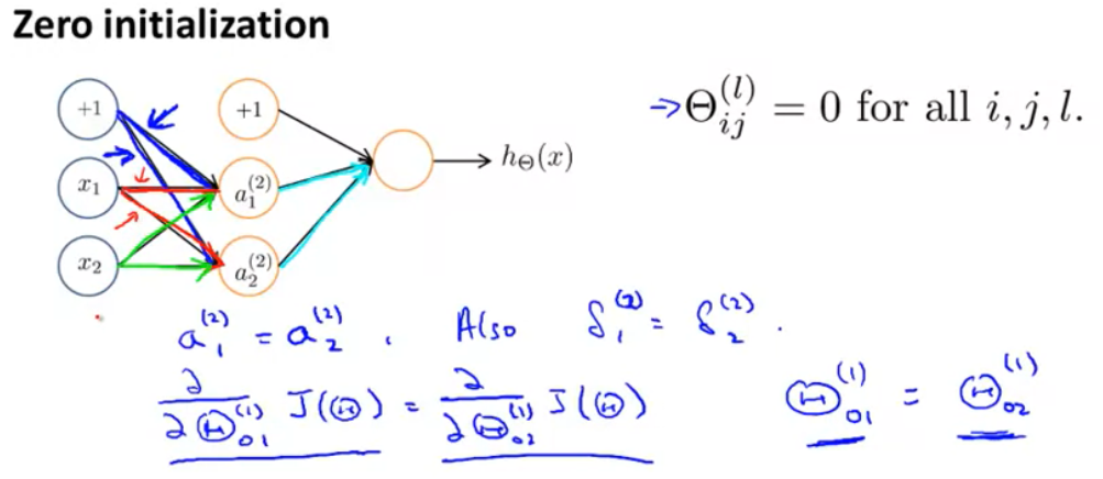
Last but not least, random initialization is very important in the programming. Zero initialization won’t give us a right solution since the gradient for each \(\Theta^{(l)}\) will be exactly the same. Details chould be checked in Week 5, Machine Learning in Coursera.

This article shows the alternative for initialization such as He initialization. I will try to explore why He initialization works better latter.